
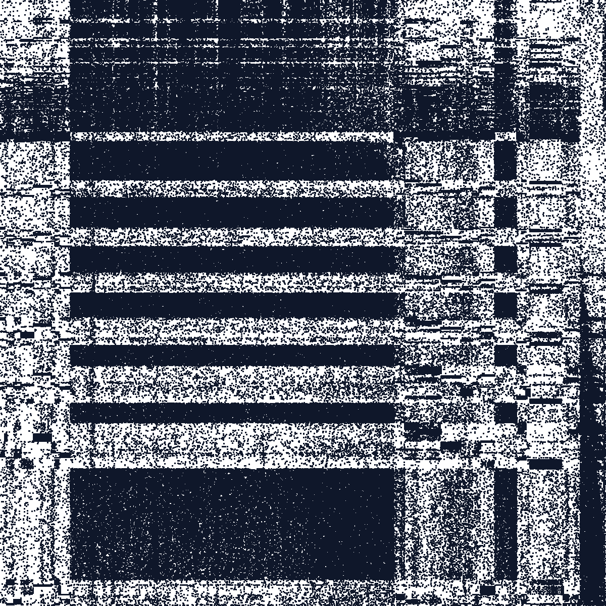
Credit, Small Subsample
A small borrower-period panel derived from the credit dataset. It is useful as a fast smoke test for HDFE implementations.
19,094rows
19,094edges
601id1 levels
140id2 levels
HDFE benchmark collection
A curated collection of datasets (CSV, Stata) for evaluating algorithms that absorb millions of fixed effects across multiple levels.
Modern empirical work often needs regressions of the form y = Xb + D a + e, where D is not one fixed effect but a collection of high-dimensional indicator matrices: workers and firms, borrowers and months, students and teachers, senders and receivers, etc. The coefficients on X are usually the object of interest, but the nuisance fixed effects can dominate the computational problem.
The standard trick is Frisch-Waugh-Lovell residualization: partial out the fixed effects from y and each column of X, then run the low-dimensional regression. For one fixed effect this is just demeaning. For two or more fixed effects it becomes an iterative numerical problem whose difficulty is governed less by the number of rows than by the connectivity of the underlying graph.
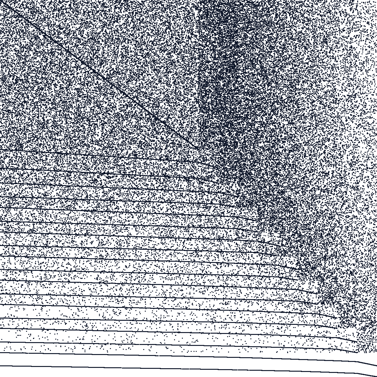
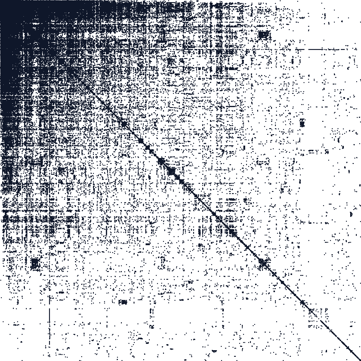
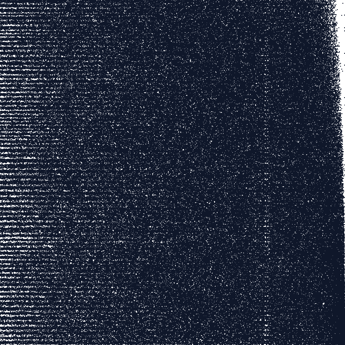
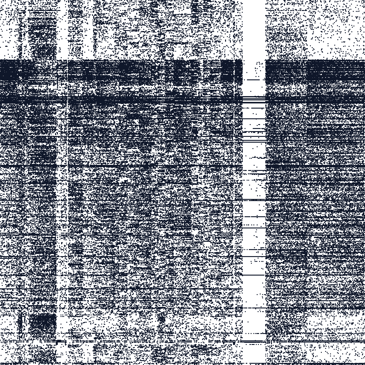
The figures below illustrate the sparsity sparsity patterns of the different datasets. They show the binned bipartite incidence blocks induced by the primary two-way fixed effects, i.e. the off-diagonal structure of the graph Laplacian. Dense, compact patterns are usually easy. Long thin structures, many separated blocks, or weak bridges are warning signs: they indicate poor algebraic connectivity, large finite condition numbers, and slow residualization for some algorithms.
A small borrower-period panel derived from the credit dataset. It is useful as a fast smoke test for HDFE implementations.

Borrower-month observations from a credit panel, with synthetic regressors and outcome added for benchmarking.

Player co-appearance data constructed from soccer match rosters, with synthetic regressors and outcome.

A complete bipartite synthetic benchmark where every unit in the first partition is matched to every unit in the second partition.

Uniform random matching synthetic benchmark with easy connectivity.

Uniform random matching synthetic benchmark with weaker connectivity.

Uniform random matching synthetic benchmark with the weakest v1 uniform connectivity.
Synthetic CEO-firm panel with turnover, retirement, poaching, and assortative matching between CEO and firm types.

A small synthetic graph designed to create a path-like hard connectivity pattern.
Email sender-recipient graph derived from the SNAP Enron email network.

Open-source contribution data derived from the Google BigQuery GitHub public dataset, with synthetic regressors and outcome.
Patent citation graph derived from the SNAP patent citation dataset.
Employer-employee matched data with anonymized firm and worker identifiers plus job-title and year fields.

Student-teacher longitudinal data with anonymized identifiers and synthetic regressors/outcome.
Firm-director matched records with synthetic regressors and outcome.
The canonical v1 figure for every dataset uses id1 and id2, because two-way fixed effects have a direct graph/Laplacian interpretation. Several datasets also include other identifier-like columns that can support richer three-way or multi-way benchmarks.
| Dataset | Primary graph | Additional identifier-like columns |
|---|---|---|
| Credit, Small Subsample | id1, id2 | ruc, t |
| Credit | id1, id2 | ruc, t |
| Soccer | id1, id2 | None in the clean v1 CSV |
| Synthetic Complete | id1, id2 | None in the clean v1 CSV |
| Synthetic Uniform, Easy | id1, id2 | None in the clean v1 CSV |
| Synthetic Uniform, Hard | id1, id2 | None in the clean v1 CSV |
| Synthetic Uniform, Harder | id1, id2 | None in the clean v1 CSV |
| Synthetic Assortative Matching | id1, id2 | year, ceo_type, firm_type |
| Synthetic Zigzag | id1, id2 | None in the clean v1 CSV |
| Enron Email | id1, id2 | None in the clean v1 CSV |
| GitHub Contributions | id1, id2 | id3, t |
| Patent Citations | id1, id2 | None in the clean v1 CSV |
| Workers | id1, id2 | id3, id4 |
| Schools | id1, id2 | id3 |
| Directors | id1, id2 | None in the clean v1 CSV |
The table below reproduces the initial benchmark timings from this project (see presentation link below). They show the central lesson of the collection (as of early 2026): no single method wins uniformly, and the hard cases are exactly the ones with weak graph connectivity.
| Dataset | MAP-Aitken | MAP-SD | MAP-CG-Sym | MAP+Prune | LSMR | Fastest |
|---|---|---|---|---|---|---|
| Synthetic-complete | 2.3 | 2.5 | 3.5 | 7.5 | 2.8 | MAP-Aitken (2.3s) |
| Synthetic-unif-easy | 7.4 | 5.0 | 4.9 | 16.8 | 10.4 | MAP-CG-Sym (4.9s) |
| Synthetic-unif-hard | 19.0 | 21.8 | 16.1 | 22.7 | 32.1 | MAP-CG-Sym (16.1s) |
| Synthetic-unif-harder | 83.5 | 49.8 | 47.2 | 50.0 | 124.2 | MAP-CG-Sym (47.2s) |
| Synthetic-assortative | 320.6 | 108.7 | 101.8 | 73.6 | 206.6 | MAP+Prune (73.6s) |
| Credit | 15.1 | 20.5 | 14.2 | 28.2 | 17.3 | MAP-CG-Sym (14.2s) |
| Enron | 51.4 | 38.1 | 29.7 | 31.5 | 51.0 | MAP-CG-Sym (29.7s) |
| Schools | 221.5 | 79.7 | 61.7 | 116.6 | 132.0 | MAP-CG-Sym (61.7s) |
| Github | 268.7 | 110.1 | 114.4 | 127.1 | 169.6 | MAP-SD (110.1s) |
| Workers | 484.1 | 146.0 | 169.6 | 646.1 | 356.3 | MAP-SD (146.0s) |
| Patents | 574.2 | 191.7 | 188.5 | 172.3 | 490.6 | MAP+Prune (172.3s) |
| Directors | 688.8 | 215.6 | 258.6 | 240.7 | 894.1 | MAP-SD (215.6s) |
To recreate comparable timings with current Stata and current packages, download benchmark_reghdfe_variants.do and run it after downloading the Stata files. For the original motivation, examples, and discussion behind these benchmarks, see the 2017 SEC presentation: Linear Models with Multi-Way Fixed Effects.